User Acquisition Analytics

Organizations have until recently done most of their user acquisition analytics on structured data. Vector embeddings have changed this. Vectors capture the semantic meaning and context of unstructured data such as text, providing more nuanced and detailed insights to inform user acquisition analysis - enabling organizations to create more strategic marketing and sales campaigns.

In this article, we'll show you how to use the Superlinked library to leverage vector embedding power to identify and analyze users on the basis of how they respond to particular ad messaging, target them more precisely, and improve conversion rates in your campaigns.

You can implement each step below as you read, in the corresponding notebook and colab.

By capturing intricate relationships and patterns between data points, and representing them as high-dimensional vectors in a latent space, embeddings empower you to extract deeper insights from complex datasets. With smart vectors, you can do more nuanced analysis, interpretation, and accurate predictions to inform your ad campaign decision-making.

Superlinked's framework lets you create vectors that are smarter representations of your data, empowering you to retrieve high quality, actionable insights (e.g., understanding why different ad creatives attract different users) without postprocessing or reranking.

Let's walk through how you can perform user acquisition analysis on ad creatives using Superlinked library elements, namely:

Recency space - encodes when a data point occurred (e.g., users' signup date) Number space - encodes the frequency of a data event (e.g., subscribed users' API calls/day) TextSimilarity space - encodes the semantic meaning of text data (e.g., campaign ad_creative text)

We have data from two 2023 ad campaigns - one from August (with more generic ad messages), and another from December (assisted by a made-up influencer, "XYZCr$$d"). Our data (for 8000 users) includes:

1. user signup date, as unix timestamp
2. the ad creative a user clicked on before signing up
3. average daily activity (for users who signed up by clicking on a campaign ad_creative), measured in api calls/day (over the user's lifetime)

We want to know which creatives bring in what kinds of users, so we can create ad messaging that attracts and retains active users. By embedding our data into a vectorspace using Superlinked Spaces, we're able to cluster users, find meaningful groups, and use a UMAP visualization to examine the relationship between cluster labels and features of our ad creatives.

Let's get started.

First, we install superlinked and umap.

%pip install superlinked==9.47.1
%pip install umap-learn

Next, we import all our dependencies and declare our constants.

import os
import sys

from datetime import datetime, timedelta
from typing import Any

import altair as alt
import numpy as np
import pandas as pd
import umap

from sklearn.cluster import HDBSCAN

from superlinked.evaluation.charts.recency_plotter import RecencyPlotter
from superlinked.evaluation.vector_sampler import VectorSampler
from superlinked.framework.common.dag.context import CONTEXT_COMMON, CONTEXT_COMMON_NOW
from superlinked.framework.common.dag.period_time import PeriodTime
from superlinked.framework.common.embedding.number_embedding import Mode
from superlinked.framework.common.parser.dataframe_parser import DataFrameParser
from superlinked.framework.common.schema.schema import Schema
from superlinked.framework.common.schema.schema_object import String, Float, Timestamp
from superlinked.framework.common.schema.id_schema_object import IdField
from superlinked.framework.common.util.interactive_util import get_altair_renderer
from superlinked.framework.dsl.executor.in_memory.in_memory_executor import (
    InMemoryExecutor,
    InMemoryApp,
)
from superlinked.framework.dsl.index.index import Index
from superlinked.framework.dsl.source.in_memory_source import InMemorySource
from superlinked.framework.dsl.space.text_similarity_space import TextSimilaritySpace
from superlinked.framework.dsl.space.number_space import NumberSpace
from superlinked.framework.dsl.space.recency_space import RecencySpace


alt.renderers.enable(get_altair_renderer())
alt.data_transformers.disable_max_rows()
pd.set_option("display.max_colwidth", 190)
pd.options.display.float_format = "{:.2f}".format
np.random.seed(0)

Here's where we declare constants.

DATASET_REPOSITORY_URL: str = (
    "https://storage.googleapis.com/superlinked-notebook-user-acquisiton-analytics"
)
USER_DATASET_URL: str = f"{DATASET_REPOSITORY_URL}/user_acquisiton_data.csv"
NOW_TS: int = int(datetime(2024, 2, 16).timestamp())
EXECUTOR_DATA: dict[str, dict[str, Any]] = {
    CONTEXT_COMMON: {CONTEXT_COMMON_NOW: NOW_TS}
}

Let's read our dataset, and then take a closer look at it:

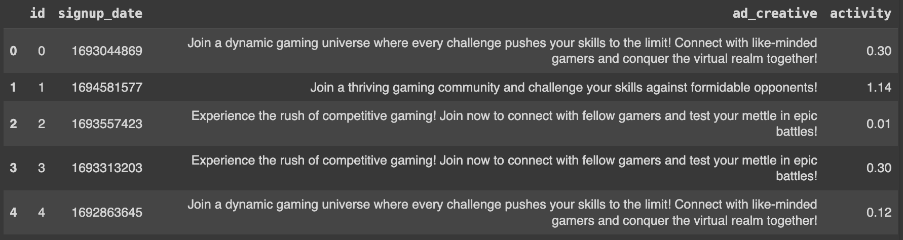
NROWS = int(os.getenv("NOTEBOOK_TEST_ROW_LIMIT", str(sys.maxsize)))
user_df: pd.DataFrame = pd.read_csv(USER_DATASET_URL, nrows=NROWS)
print(f"User data dimensions: {user_df.shape}")
user_df.head()

We have 8000 users, and (as we can see from the first five rows) 4 columns of data:

To understand which ad creatives generated how many signups, we create a DataFrame:

pd.DataFrame(user_df["ad_creative"].value_counts())

...which looks like this:

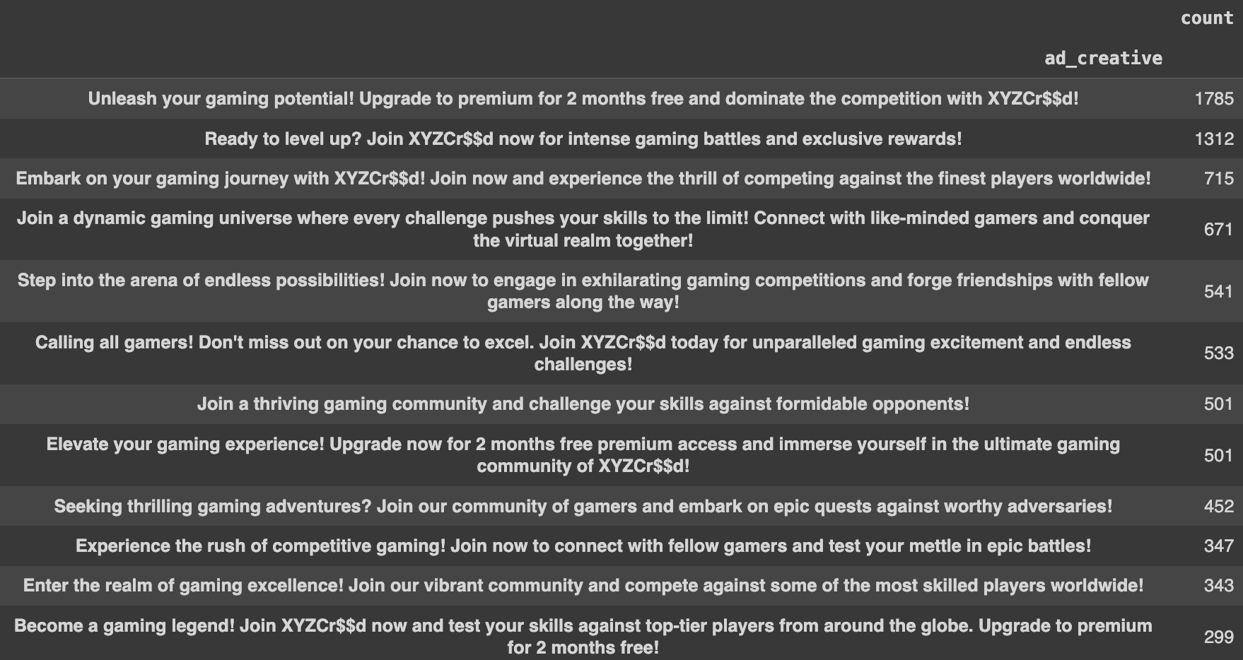
The influencer (XYZCr$$d) backed ad creatives seem to have worked better - generating many more signups (total 5145) than the August campaign ad creatives (total 2855).

Now, let's take a look at the distribution of users by activity level (api calls/day).

alt.Chart(user_df).mark_bar().encode(
    alt.X("activity:Q", bin=True, title="Activity count"),
    alt.Y("count()", title="# of users"),
).properties(width=600, height=400)

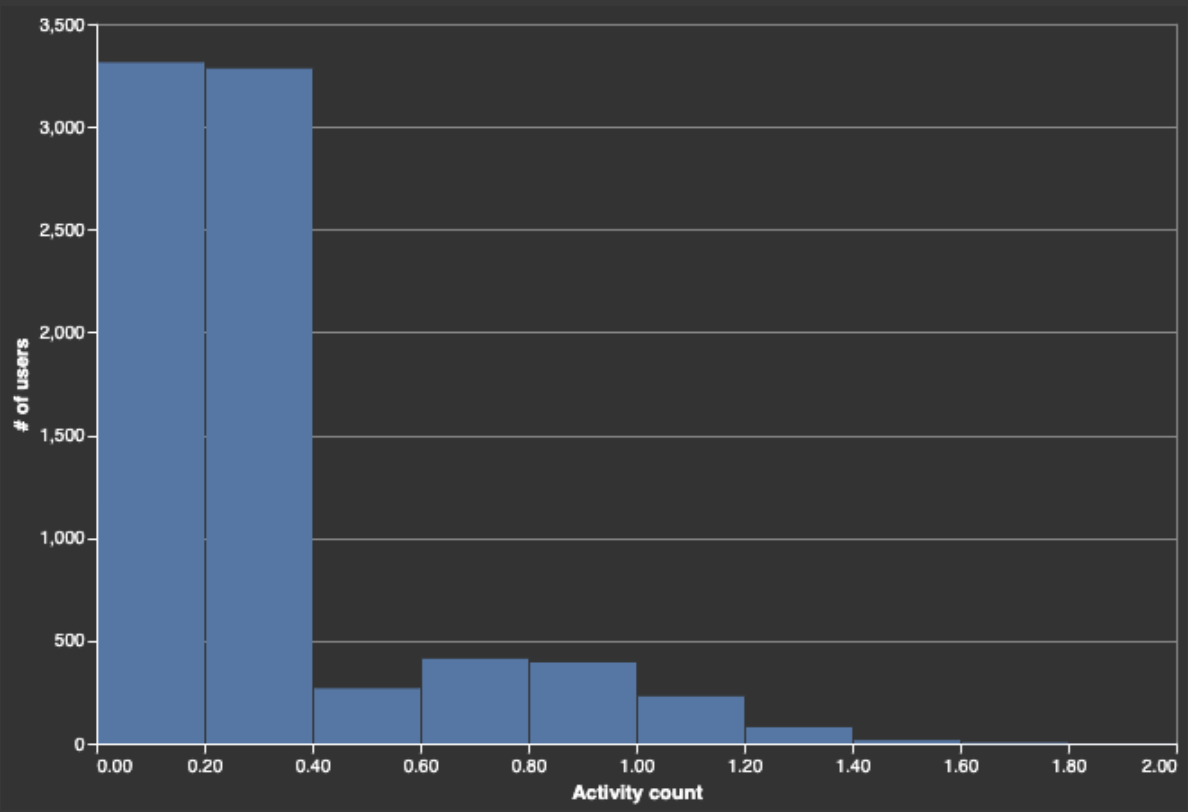
The activity (api calls/day) distribution is bimodal. Most users are either inactive or have very low activity levels - i.e., they signed up, maybe performed a few actions and then never returned, or returned only occasionally after clicking on a subsequent campaign. The active users distribution has a mode around 0.6-0.8 api calls/day - i.e., returning every 2-3 days, triggering 1-2 api calls/day. (Note: we can also use this activity distribution to derive our NumberSpace min and max.)

Now let's examine the distribution of new users per signup date.

dates: pd.DataFrame = pd.DataFrame(
    {"date": [str(datetime.fromtimestamp(ts).date()) for ts in user_df["signup_date"]]}
)
dates_to_plot = pd.DataFrame(dates.value_counts(), columns=["count"]).reset_index()
alt.Chart(dates_to_plot).mark_bar().encode(
    alt.X("date", title="Signup date"), alt.Y("count", title="Number of subscribers")
).properties(height=400, width=1200)

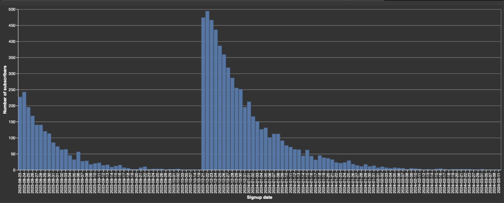
This distribution confirms that our second campaign (December) works much better than the first (August). The jump in signups at 2023-12-21 coincides with our second campaign, and our data is exclusively users who signed up by clicking on campaign ad_creatives. To get more insights from our user acquisition analysis, we need two periods that fit our distribution. A first period of 65 days and a second of 185 days seem appropriate.

Of our 8k users, roughly 2k subscribed in the first campaign period (65 days), and 6k in the second. Since we already know which ad_creatives users clicked on to go sign up (2855 on old campaign ads, 5145 on new campaign ads), we know that some of the roughly 6k users clicked on old (August) campaign ads after the new (December) campaign ad began (possibly after seeing the new campaign ads).

Here's what we've established so far:

• that many more users signed up in response to the influencer-backed ad creatives (second campaign) than the first
• which specific ad creatives generated the most user signups
• that the vast majority of users have low to moderate activity

We don't know:

• which ad creatives resulted in low vs medium vs high activity users?
• how did users cluster in terms of signup date, activity levels, and ad_creatives they clicked?
• are there user data patterns we can mine to make better decisions when planning our next campaign?

Fortunately, embedding with Superlinked spaces will help provide answers to these questions, empowering us to adopt a more effective user acquisition strategy.

Now, let's use Superlinked to embed our data in a semantic space, so that we can:

1. inform our model as to which ad creatives generated signups, and which users (with specific activity level distributions) signed up
2. group specific ad creatives that have similar meanings, and possibly outcomes

First, we define a schema for our user data:

class UserSchema(Schema):
    ad_creative: String
    activity: Float
    signup_date: Timestamp
    id: IdField

user = UserSchema()

Now we create a semantic space for our ad_creatives using a text similarity model. Then, we encode user activity into a numerical space to represent users' activity level. We also encode the signup date into a recency space, allowing our clustering algorithm to take account of the two specific periods of signup activity (following our two campaign start dates).

# create a semantic space for our ad_creatives using a text similarity model
creative_space = TextSimilaritySpace(
    text=user.ad_creative, model="sentence-transformers/all-mpnet-base-v2"
)

# encode user activity into a numerical space to represent users' activity level
activity_space = NumberSpace(
    number=user.activity, mode=Mode.SIMILAR, min_value=0.0, max_value=1.0
)

# encode the signup date into a recency space
recency_space = RecencySpace(
    timestamp=user.signup_date,
    period_time_list=[PeriodTime(timedelta(days=65)), PeriodTime(timedelta(days=185))],
    negative_filter=0.0,
)

Let's plot our recency scores by date.

recency_plotter = RecencyPlotter(recency_space, context_data=EXECUTOR_DATA)
recency_plotter.plot_recency_curve()

Next, we set up an in-memory data processing pipeline for indexing, parsing, and executing operations on user data.

First, we create our index with the spaces we use for clustering.

user_index = Index(spaces=[creative_space, activity_space, recency_space])

Now for dataframe parsing.

user_df_parser = DataFrameParser(schema=user)

We create an InMemorySource object to hold the user data in memory, and set up our executor (with our user data source and index) so that it takes account of context data. The executor vectorizes based on the index's grouping of Spaces.

source_user: InMemorySource = InMemorySource(user, parser=user_df_parser)
executor: InMemoryExecutor = InMemoryExecutor(
    sources=[source_user], indices=[user_index], context_data=EXECUTOR_DATA
)
app: InMemoryApp = executor.run()

Now we input our user data.

source_user.put([user_df])

(The step above make take a few minutes or more. In the meantime, why not learn more about vectors in Vectorhub.)

Next, we collect all our vectors from the app. The vector sampler helps us export vectors so we can cluster and (umap) visualize them.

vs = VectorSampler(app=app)
vector_collection = vs.get_all_vectors(user_index, user)
vectors = vector_collection.vectors
vector_df = pd.DataFrame(vectors, index=[int(id_) for id_ in vector_collection.id_list])
vector_df.head()

vector_df.shape

Here are the first five rows (of 8000), and 776 columns, of the resulting dataframe:

Next, we fit a clustering model.

hdbscan = HDBSCAN(min_cluster_size=500, metric="cosine")
hdbscan.fit(vector_df.values)

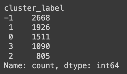
Let's create a DataFrame to store the cluster labels assigned by HBDSCAN and count how many users belong to each cluster:

label_df = pd.DataFrame(
    hdbscan.labels_, index=vector_df.index, columns=["cluster_label"]
)
label_df["cluster_label"].value_counts()

Let's try to interpret our dataset by visualizing it using UMAP.

First, we'll fit the UMAP and transform our dataset:

umap_transform = umap.UMAP(random_state=0, transform_seed=0, n_jobs=1, metric="cosine")
umap_transform = umap_transform.fit(vector_df)
umap_vectors = umap_transform.transform(vector_df)
umap_df = pd.DataFrame(
    umap_vectors, columns=["dimension_1", "dimension_2"], index=vector_df.index
)
umap_df = umap_df.join(label_df)

Next, we join our dataframes and create a chart, letting us visualize the UMAP-transformed vectors, and color them with cluster labels.

alt.Chart(umap_df).mark_circle(size=8).encode(
    x="dimension_1", y="dimension_2", color="cluster_label:N"
).properties(
    width=600, height=500, title="UMAP Transformed vectors coloured by cluster labels"
).configure_title(
    fontSize=16,
    anchor="middle",
).configure_legend(
    strokeColor="black",
    padding=10,
    cornerRadius=10,
    labelFontSize=14,
    titleFontSize=14,
).configure_axis(
    titleFontSize=14, labelFontSize=12
)

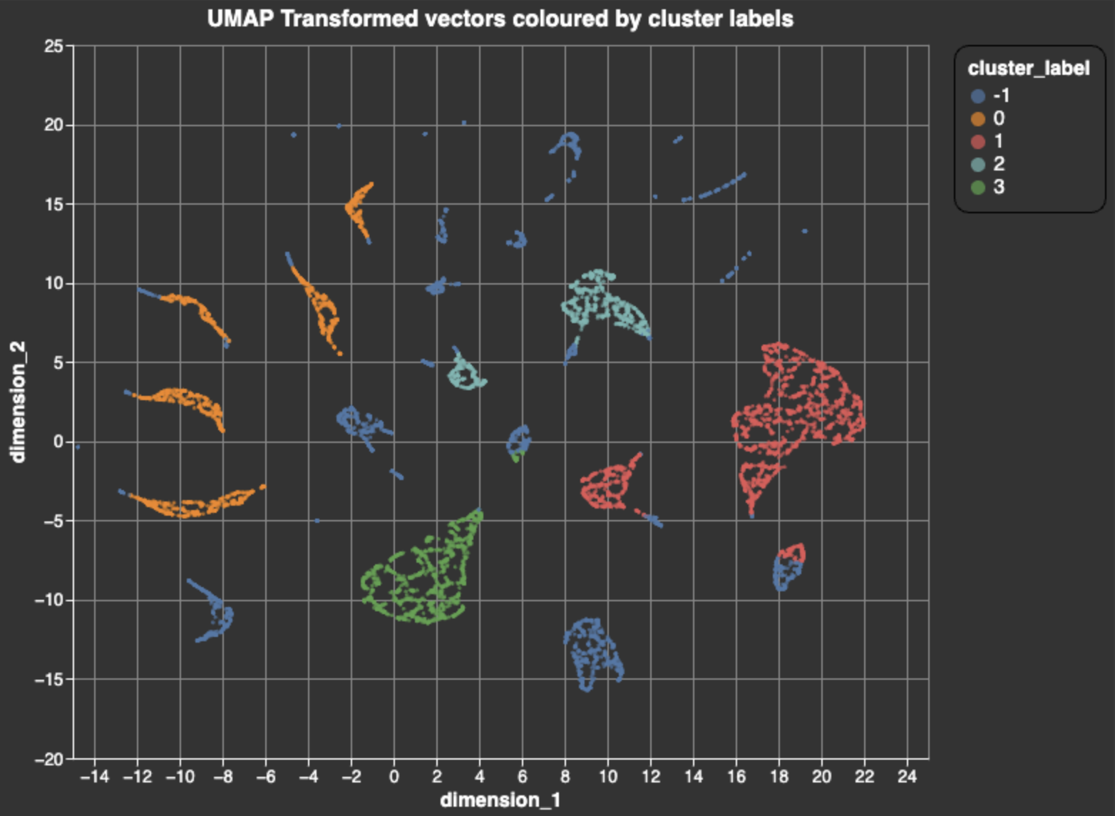
The dark blue clusters (label -1) are outliers - not large or dense enough to form a distinct group. Our data points are represented by vectors with three attributes (signup recency, ad_creative textSimilarity, and signed up user activity level), each attribute accounting for 1/3 of each vector's mass. The limited number of discrete ad_creatives (13), then, tends towards producing more distinct blobs in the umap visualization of the vector space, whereas signup_date and activity level are more continuous variables, and tend towards producing more dense blobs. *Note: 2D (UMAP) visualizations can make some clusters look quite dispersed / scattered.

To understand our user clusters better, we can produce some activity histograms.

First, we join user data with cluster labels, create separate DataFrames for each cluster, generate activity histograms for each cluster, and then concatenate these histograms into a single visualization.

# activity histograms by cluster
user_df = user_df.set_index("id").join(label_df)

by_cluster_data = {
    label: user_df[user_df["cluster_label"] == label]
    for label in np.unique(hdbscan.labels_)
}

activity_histograms = [
    alt.Chart(user_df_part)
    .mark_bar()
    .encode(
        x=alt.X("activity", bin=True, scale=alt.Scale(domain=[0, 1.81])),
        y=alt.Y("count()", scale=alt.Scale(domain=[0, 1000])),
    )
    .properties(title=f"Activity histogram for cluster {label}")
    for label, user_df_part in by_cluster_data.items()
]

alt.hconcat(*activity_histograms)

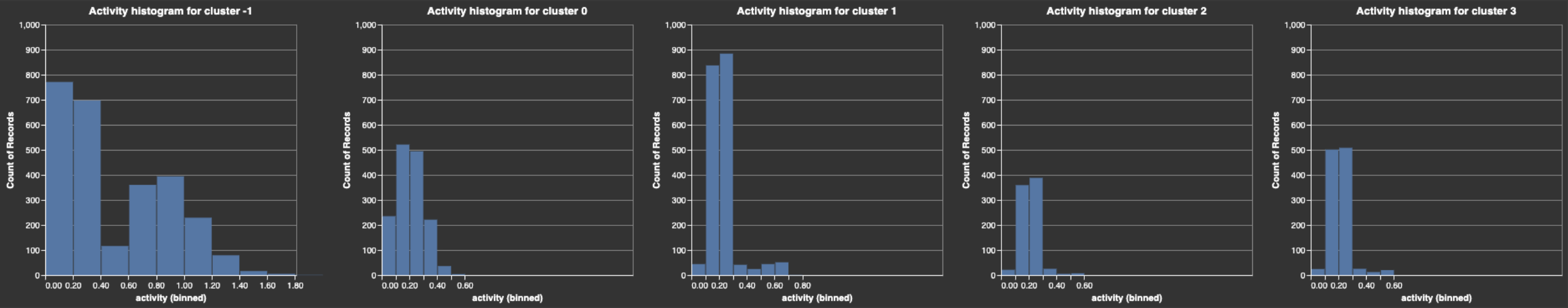
Our users' activity profiles conform to a power-law distribution that's common in user activity profiles: most users tend to be low activity, some medium activity, and very active users quite rare.

From our histograms, we can observe that:

• cluster -1 users are outliers, not dense enough to form a proper cluster - balanced, with predominantly low, a few medium, and all the most active users
• cluster 0 has mostly low-moderate activity users, and the lowest number of (i.e., nearly zero) highly active users
• cluster 1 has the most low-moderate/medium activity users, and the second largest number of highly active users (next to the outliers cluster (-1))
• clusters 2 and 3 are predominately low-moderate activity users, with a few medium activity users

To see the distribution of ad_creatives across different clusters, we create a DataFrame that shows each ad_creative's count value within each cluster:

pd.DataFrame(user_df.groupby("cluster_label")["ad_creative"].value_counts())

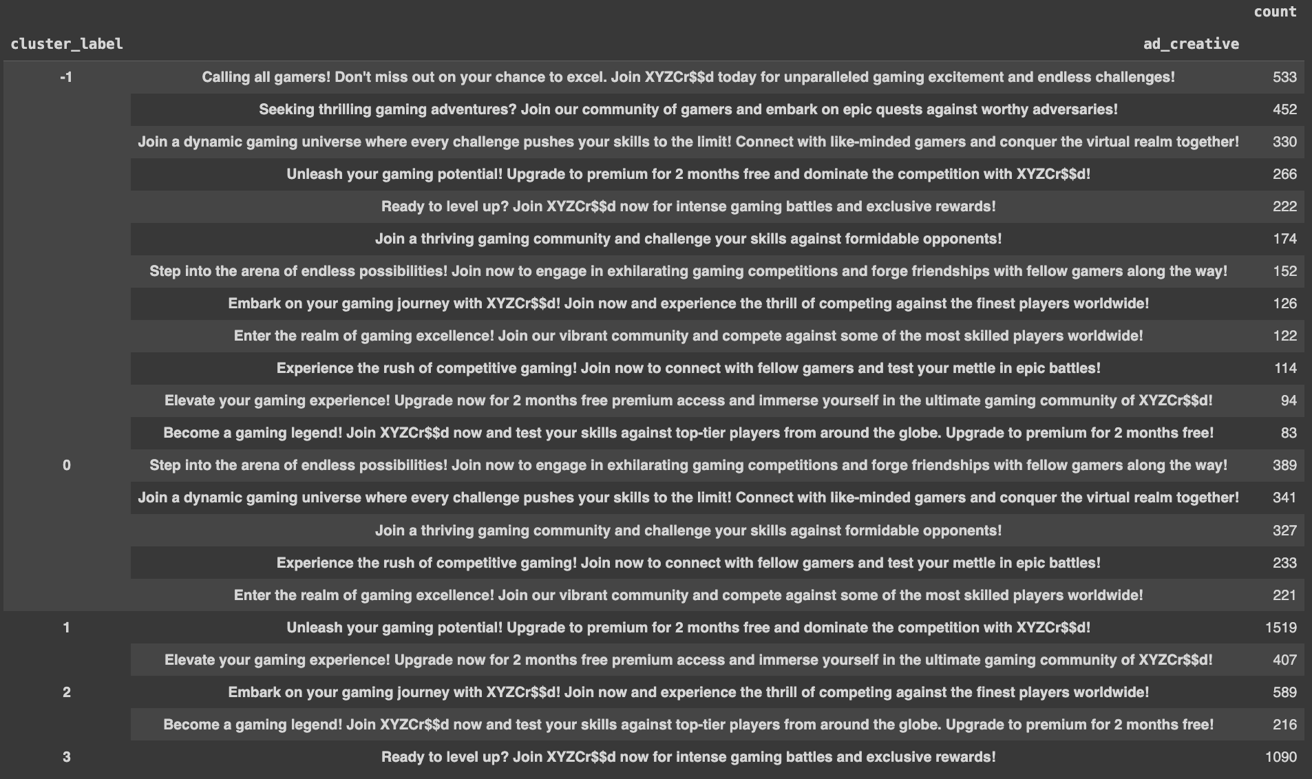
What can we observe here?

• cluster -1 (with the most high and extremely high activity users) clicked on ad_creatives from both campaigns (as expected); 1324 clicks on new campaign ads, 1344 on old
• cluster 0 clicked on only the first (non-influencer) campaign; these ads focus on community and competition within the gaming platform
• clusters 1 and 2 clicked on only two influencer campaign ad creatives each; cluster 1 ads focused on the benefits of premium membership; cluster 2 ads highlighted experience and achievement in the gaming platform
• cluster 3 clicked on only one ad_creative - from the influencer campaign; this ad was an immediate appeal based on promised excitement and the exclusive rewards of joining

Now, let's get some descriptive stats for our signup dates to help us interpret our clusters' behavior further.

user_df["signup_datetime"] = [
    datetime.fromtimestamp(ts) for ts in user_df["signup_date"]
]
desc = user_df.groupby("cluster_label")["signup_datetime"].describe()
for col in desc.columns:
    if col == "count":
        continue
    desc[col] = [dt.date() for dt in desc[col]]
desc

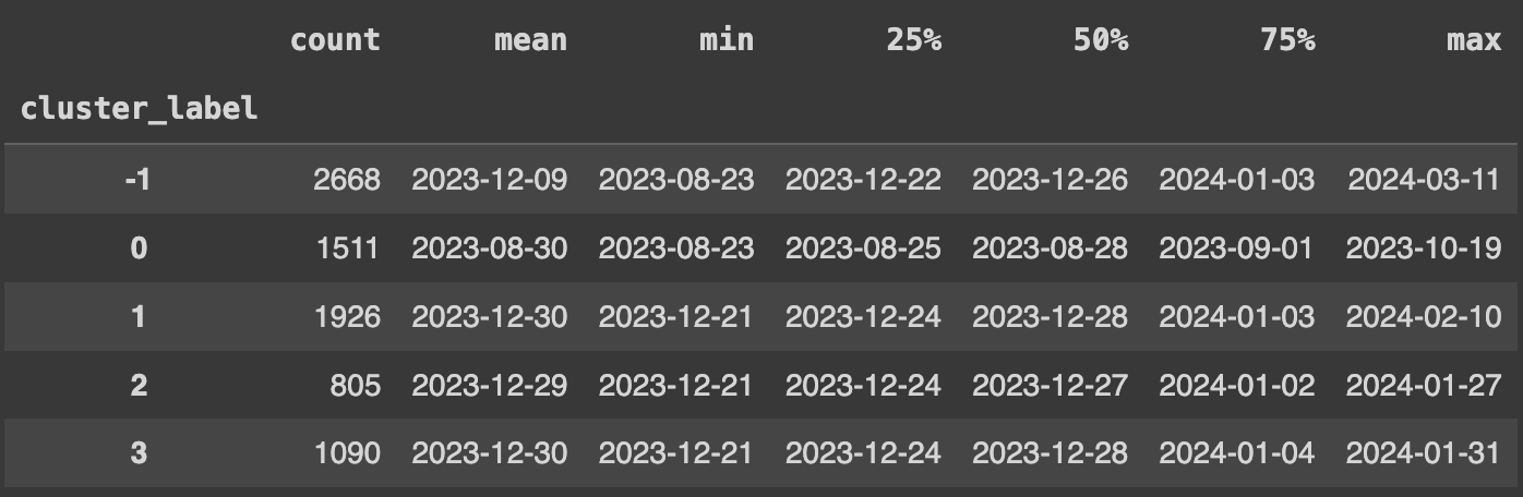
What do our clusters' signup dates data indicate?

• outliers' (cluster -1) have signup dates that are scattered across both campaign periods
• cluster 0's signups came entirely from clicks on the first campaign's ad_creatives
• clusters 1, 2, and 3 signed up in response to the new (influencer-augmented) campaign only

Let's summarize our findings.

Overall, the influencer-backed (i.e., second) campaign performed better. Roughly 58% of user signups came exclusively from clicks on second campaign ad_creatives. These ads were influencer-based, included a call to action, emphasized benefits, and had motivating language. (Two ads in particular accounted for 38% of all signups: "Unleash your gaming potential! Upgrade to premium for 2 months free and dominate the competition with XYZCr$$d!" (22%), and "Ready to level up? Join XYZCr$$d now for intense gaming battles and exclusive rewards!" (16%).)

Users who signed up in response to ads that focused on enhanced performance, risk-free premium benefits, and community engagement - cluster 1 - tended to be predominantly medium activity users, but also included a nontrivial number of low and high activity users. Cluster 1 users also made up the largest segment of subscriptions (35%). Both these findings suggest that this kind of ad_creative provides the best ROI.

Cluster 0, though its users signed up exclusively in response to the first (non-influencer) campaign, is still relatively low to medium activity - its overall distribution is left of clusters 1, 2, and 3 - suggesting that users who subscribe in response to the non-influencer campaign ads are less active than users who signup after clicking on new campaign ads. Still, we need to continue monitoring user activity to see if these patterns hold over time.

Using Superlinked's Number, Recency, and TextSimilarity Spaces, we can embed various aspects of our user data, and create clusters on top our vector embeddings. By analyzing these clusters, we reveal patterns previously invisible in the data - which ad_creatives work well at generating signups, and how users behave after signups resulting from certain ad_creatives. These insights are invaluable for shaping more strategic marketing and sales decisions.

Now it's your turn. Experiment with the Superlinked library yourself in the notebook!